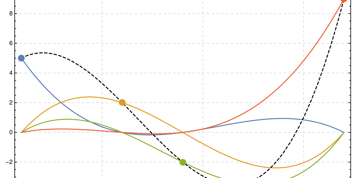
Lagrange interpolating polynomials

Here is the Lagrange interpolating polynomial equation:

$L_i(X)=\prod_{j=0\atop j \ne i}^n\frac{(X-a_j)}{(a_i-a_j)}$

$\boxed{P=\sum_{i=0}^nP(a_i)L_i(X)}$

You can find a python code hosted in GitHub here: https://github.com/eddydu44/Lagrange-interpolating-polynomials

It calculates the polynomial that passes through points given interactively.

And it plots a graph like these ones :

Code :

from functools import reduce
from sympy import Symbol
X = Symbol('X')
def Lagrange(points):
 P=[reduce((lambda x,y: x*y),[(X-points[j][0])/(points[i][0] - points[j][0]) for j in range(len(points)) if i != j])*points[i][1] for i in range(len(points))]
 return sum(P)
print("Enter every points in this format : x y \nStop the list by entering 0")
p1=0
points=[]
while True:
 p1 = [int(x) for x in input("Enter point coord: ").split()]
 if p1 == [0]:
 break
 points+=[p1]
print(points)
P=Lagrange(points)
print("\nLagrange equation :\n")
print(P)
import matplotlib.pyplot as plt
from numpy import arange
def graph(P,points):
 plt.plot([points[i][0] for i in range(len(points))], [points[i][1] for i in range(len(points))], 'ro')
 plt.title('P(X)=' + str(P))
 xmin=min([points[i][0] for i in range(len(points))])-1
 xmax=max([points[i][0] for i in range(len(points))])+1
 t1 = arange(xmin, xmax, 0.02)
 def f(t):
 t2 = []
 for i in t :
 t2 += [P.subs(X,i)]
 return t2
 plt.plot(t1,f(t1),'r--')
 plt.show()
graph(P,points)

Lagrange interpolating polynomials

AUTEUR

eddy barraud

Laissez un commentaire Annuler la réponse